Representing Exponential Decay
Student Summary
Here is a graph showing the luminescence of a glow-in-the-dark paint, measured in lumens, over a period of time, measured in hours. The luminescence of this glow-in-the-dark paint can be modeled by an exponential function.
Notice that the amounts are decreasing over time. The graph includes the point (0,12). This means that when the glow-in-the-dark paint started glowing, its glow measured 12 lumens. The point (1,6) tells us the glow measured 6 lumens 1 hour later. Between 3 and 4 hours after the glow-in-the-dark paint began to glow, the luminescence fell below 1 lumen.
We can use the graph to find out what fraction of luminescence stays each hour. Notice that 126=21 and 63=21. As each hour passes, the luminescence that stays is multiplied by a factor of 21.
If y is the luminescence, in lumens, and t is time, in hours, then this situation is modeled by the equation:
y=12⋅(21)t
We can confirm that the data is changing exponentially because it is multiplied by the same value each time. When the growth factor is between 0 and 1, the quantity being multiplied decreases, the situation is sometimes called “exponential decay,” and the growth factor may be called a “decay factor.”
Visual / Anchor Chart

Standards
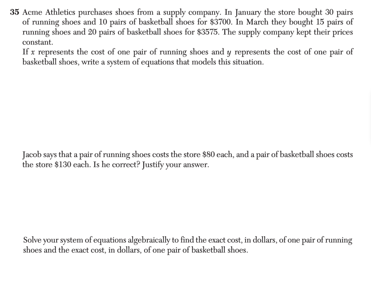
A-CED.21 question
Create equations and linear inequalities in two variables to represent a real-world context.
F-LE.53 questions
F-IF.45 questions
For a function that models a relationship between two quantities: i) interpret key features of graphs and tables in terms of the quantities; and ii) sketch graphs showing key features given a verbal description of the relationship.
F-BF.A
No additional information available.
F-LE.2
No additional information available.
F-IF.45 questions
For a function that models a relationship between two quantities: i) interpret key features of graphs and tables in terms of the quantities; and ii) sketch graphs showing key features given a verbal description of the relationship.
F-IF.7.e
Graph functions and show key features of the graph by hand and by using technology where appropriate.